2. Valence Bond Structures

In this lecture, we will introduce the concept of valence bond (VB) structures, learn what a VB structure is, and how to generate VB structures for a given system.

Before we begin today’s content, let’s think about the following questions:

Consider

How many VB structures does H₂ have? What about 1,3-butadiene? And something more complex, like naphthalene? Or the O₂ molecule?

2.1. Active Space

Let us first return to molecular orbital (MO) theory. The foundation of MO theory is the Hartree–Fock (HF) method. In the HF method, the molecular wave function is described by a single Slater determinant, where electrons occupy molecular orbitals according to the Aufbau principle, the Pauli exclusion principle, and Hund’s rule. When electrons are excited from lower-energy orbitals to higher-energy orbitals, excited determinants are generated, as shown in Fig. 2.1.1.

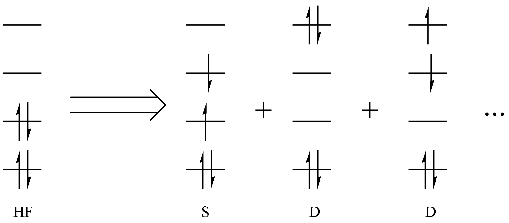
_images/excitation.png — Fig. 2.1.1 Generating excited determinants from the HF wavefunction

If only one electron is excited, this is called a single excitation (S), If two electrons are excited, it is a double excitation (D), And so on. For an n-electron system, up to n-fold excitations are possible. If we include all excitations up to the n-th order and solve for the total wave function, we obtain the Full Configuration Interaction (FCI) method. FCI is recognized as the most accurate method, but its computational cost is prohibitively high, so it is only feasible for very small systems. As a compromise, chemists usually restrict excitations to only a subset of electrons and orbitals that are relevant to the chemical problem at hand. The selected electrons and orbitals are referred to as the active space, while the corresponding electrons and orbitals are called active electrons and active orbitals, respectively (highlighted in red in Fig. 2.1.2). The remaining occupied orbitals and electrons, which do not participate in excitations and remain unchanged (fully occupied) during the process, are called the inactive space (highlighted in blue in Fig. 2.1.2).

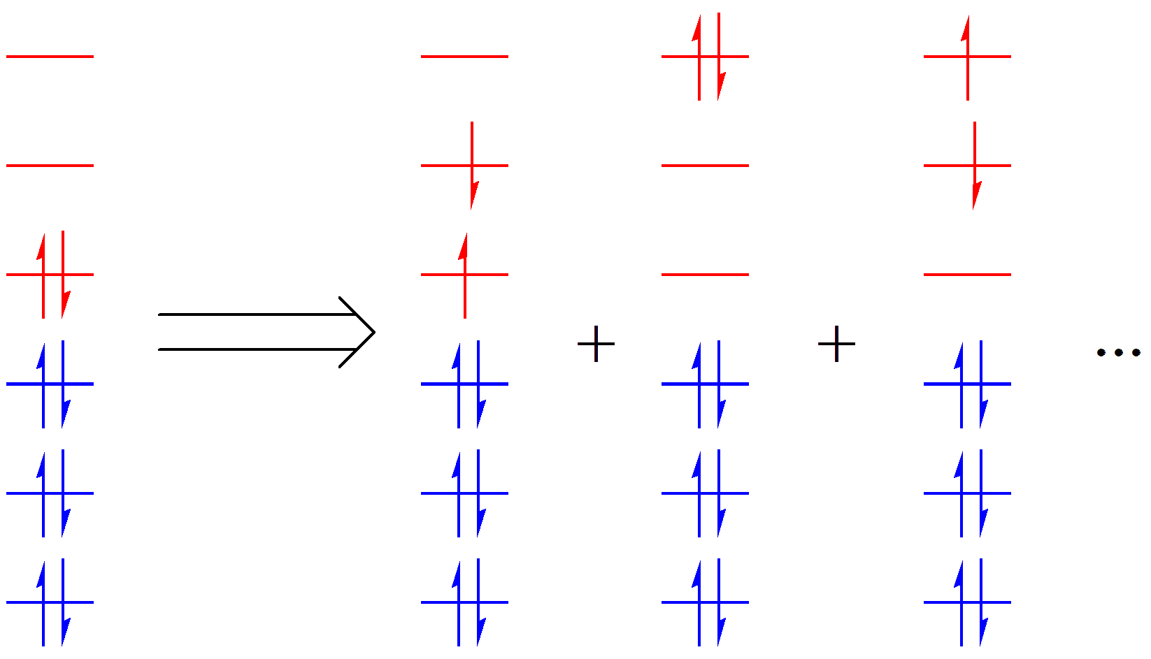
_images/active_space_mo.png — Fig. 2.1.2 Representation of the active space in molecular orbital theory

In VB theory, the concept of the active space is similar. In VB theory, depending on how electrons occupy VB orbitals, we can generate a series of VB structures. For a given system and chemical problem, we only select those VB orbitals and electrons that are directly relevant to the problem to generate VB structures. This subset of orbitals and electrons is called the active space. For example, in the VB structures of C₂ H₆ shown in Fig. 2.1.3, the red and blue regions represent the active and inactive spaces, respectively.

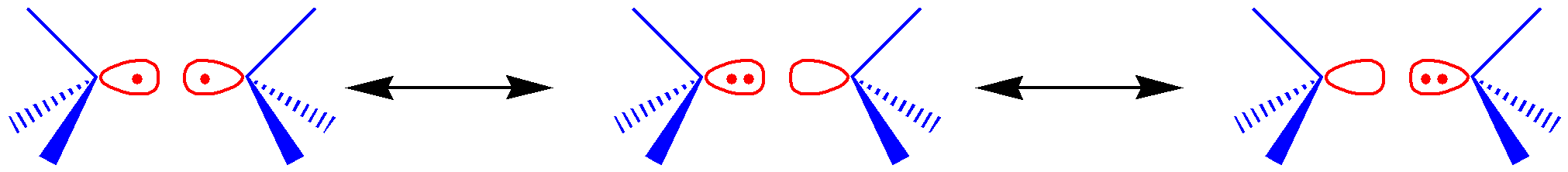
_images/active_space_vb.png — Fig. 2.1.3 Representation of the active space in valence bond theory

The active space is generally denoted as (m, n), where m is the number of active electrons and n is the number of active orbitals. For example, (2,2) means 2 active electrons in 2 active orbitals, while (8,6) means 8 active electrons in 6 active orbitals. It is important to note that the inactive space is always closed-shell. Therefore, for systems containing unpaired electrons (with spin multiplicity greater than 1), the unpaired electrons and their corresponding orbitals must also be included in the active space.

The concept of the active space is both fundamental and crucial. Not only is it essential in VB theory, but it also plays a central role in multiconfigurational self-consistent field (MCSCF) methods within MO theory—such as CASSCF (Complete Active Space SCF) and RASSCF (Restricted Active Space SCF)—where the active space specifies the number and range of electronic excitations.

2.2. Rumer’s Rule

Now that we already understand the concept of the active space, the next question is: for a given system (such as a molecule), once the active space is specified, how do we generate the required structures?

For example, in the case of the H₂ molecule, we can choose a scheme with 2 active electrons and 2 active orbitals, which leads to the 3 valence bond structures shown below:

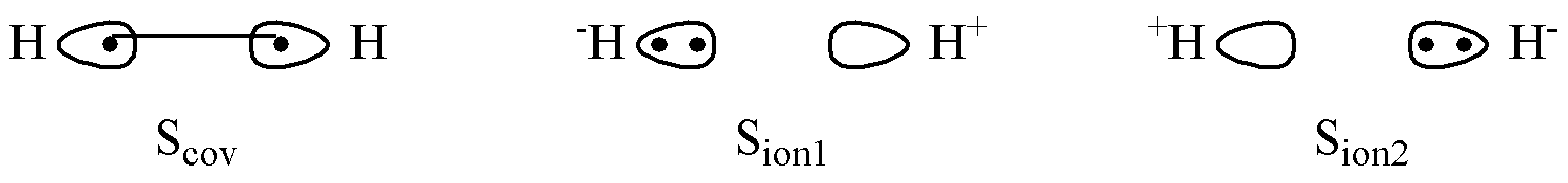
This is very straightforward and natural. For systems such as HF, F₂, and C₂ H₆, as long as we select the single bond between two atoms or groups, we can similarly obtain 3 valence bond structures. But what if the system is more complex?

For 1,3-butadiene ( C₄ H₆ ), its molecular structure is shown below:

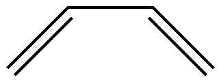
Suppose the active space consists of 4 \(\pi\)electrons and the corresponding orbitals. How do we obtain all of its valence bond structures? The simplest approach would be to list all possible configurations. By combinatorial reasoning, we can obtain the following 3 covalent structures:

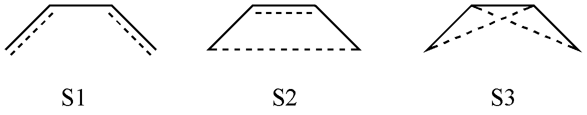
_images/c4h6_cov_wrong.png — Fig. 2.2.1 Possible covalent structures in the C₄ H₆ molecule

However, if you attempt to perform calculations using these 3 valence bond structures, you will find that the calculation fails! This is because these 3 structures are not linearly independent. In fact, it can be shown that S3 can be expressed as a linear combination of S1 and S2:

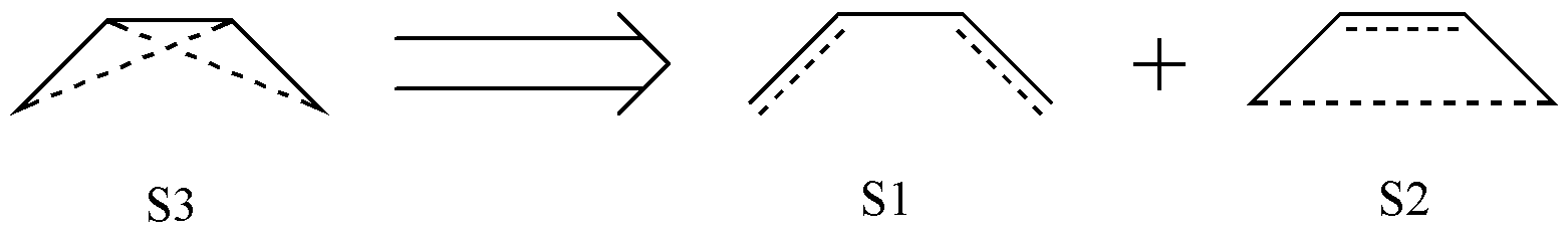
_images/c4h6_cov_linear_comb.png — Fig. 2.2.2 Linear combination among covalent structures of C₄ H₆

In fact, the C₄ H₆ molecule has only 2 covalent structures. Therefore, the valence bond structures obtained by simple combinatorial reasoning contain redundancy, and we must eliminate this redundancy before performing valence bond calculations. So how do we identify redundant structures? In other words, how can we generate valence bond structures without redundancy? This is exactly where Rumer’s rule comes into play.

2.2.1. Closed-shell case

Let us first look at the simpler closed-shell case. For a closed-shell system, all electrons are fully paired. In this case, the procedure of Rumer’s rule to generate valence bond structures is as follows:

Arrange the active orbitals in a certain order along a circle and label them with numbers;
For ionic structures, specify the positions of the doubly occupied orbital(s) and empty orbital(s);
For the remaining orbitals, pair them up in all possible ways, and then eliminate all structures with crossing lines. The remaining ones are linearly independent structures.

Let us try applying Rumer’s rule to generate the valence bond structures of C₄ H₆. First, we arrange the 4 active orbitals in a circle and label them with numbers:

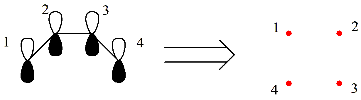
_images/c4h6_rumer_step1.png — Fig. 2.2.3 Arranging the \(\pi\)orbitals of C₄ H₆ in order

For covalent structures, we simply pair the 4 orbitals two by two:

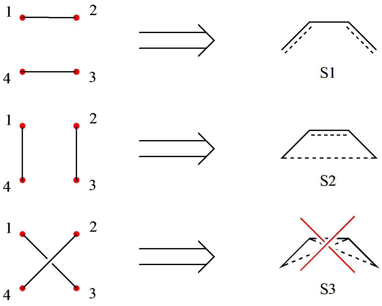
_images/c4h6_rumer_step2.png — Fig. 2.2.4 Pairing orbitals and eliminating the “crossed” case

Since S3 involves crossing lines, it must be eliminated. Thus, we obtain 2 covalent structures.

For ionic structures, suppose we now have one doubly occupied orbital and one empty orbital (i.e., one ionic pair). In this case, the positions of the ionic pair must first be fixed. Since an ionic pair is not a covalent bond, it is not subject to the “non-crossing” rule, and thus all configurations can be listed directly by simple combinatorics. In the end, we can obtain the 20 valence bond structures shown in Fig. 2.2.5, including 2 covalent structures (S1–S2), 12 first-order ionic structures (containing one ionic pair, S3–S14), and 6 second-order ionic structures (containing two ionic pairs, S15–S20).

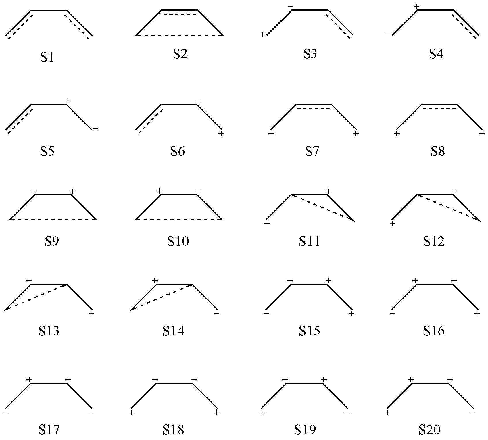
_images/c4h6_structures.png — Fig. 2.2.5 Complete valence bond structures of C₄ H₆ generated by Rumer’s rule

2.2.2. Open-shell case

In practical calculations, we often encounter many open-shell systems that contain unpaired electrons, such as various radicals. For such systems, we need to make some modifications to Rumer’s rule for the closed-shell case.

When arranging the active orbitals into a circle, we need to add an extra pole.
When drawing connections, the pole only connects to unpaired electrons, and a single pole can connect to multiple unpaired electrons;
Covalent bonds cannot cross with other covalent bonds, nor can they cross with lines involving the pole.

Let us illustrate this with the covalent structures of C₄ H₆. Suppose C₄ H₆ is in a triplet state, meaning that 2 \(\pi\)electrons are unpaired. In this case, the first step of drawing the circle becomes:

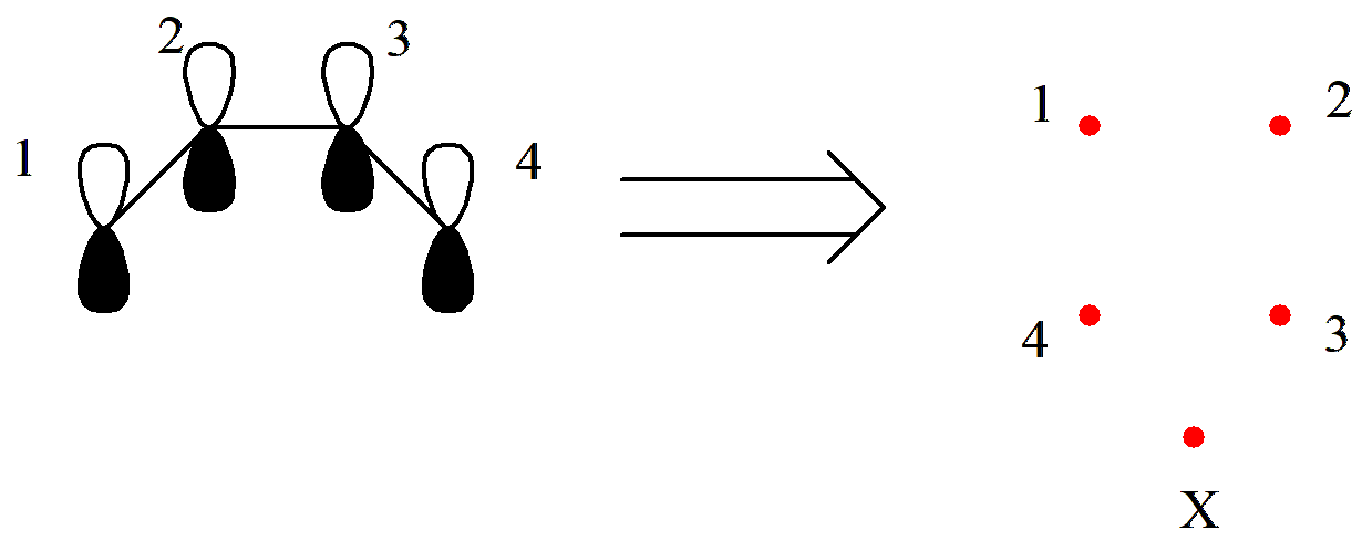
_images/c4h6_rumer_step1_triplet.png — Fig. 2.2.6 \(\pi\)Orbital arrangement of triplet C₄ H₆

Here, X represents the pole, which connects to the unpaired electrons. Next, we proceed to draw the connections:

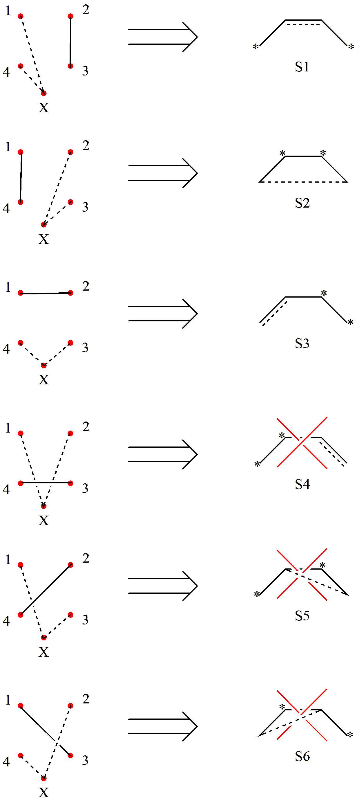
_images/c4h6_rumer_step2_triplet.png — Fig. 2.2.7 Screening covalent structures of triplet C₄ H₆

As we can see, although 6 covalent structures can be generated by combinatorics, only 3 satisfy the non-crossing rule. Therefore, triplet C₄ H₆ has 3 covalent structures. Similarly, according to Rumer’s rule, we can obtain all valence bond structures for triplet C₄ H₆.

Exercise

Use Rumer’s rule to draw:

All valence bond structures of triplet C₄ H₆.
All valence bond structures of closed-shell benzene in the \(\pi\)(6,6) active space.
All valence bond structures of the allyl radical (C₃ H₅) in the \(\pi\)(3,3) active space, as shown below.

In actual calculations, XMVB can automatically generate valence bond structures within the specified active space based on Rumer’s rule. Here, you only need to understand the underlying idea of Rumer’s rule, without worrying too much about the details.

2.3. How to interpret valence bond structures in XMVB?

In XMVB calculations, each valence bond structure is represented by a string of numbers. So how do we interpret these numbers in order to know which valence bond structures we have obtained?

In XMVB, the representation of valence bond structures is based on electron pairs. Starting from the first number, every two numbers denote the occupancy of one electron pair, with the numbers indicating the indices of the orbitals occupied by the two electrons. For a system containing a unpaired electrons (with spin multiplicity a+1), the last a numbers specify the orbitals occupied by the unpaired electrons. It should be noted that the interpretation of valence bond structures can only be completed when combined with the definition of the orbitals, since the chemical picture of the structures depends on the specific orbitals. Here, we will first explain the interpretation of valence bond structures themselves, while the definition of valence bond orbitals and the further interpretation will be covered in later chapters.

Let us first take H₂ as an example. H₂ is a closed-shell system, and all electrons are paired. The XMVB output shows that H₂ includes the following 3 valence bond structures:

  Number of structures:     3

 The following structures are used in calculation:

       1   *****     1-2
       2   *****     1 1
       3   *****     2 2

The first structure 1-2 represents an electron pair, with one electron occupying orbital 1 and the other electron occupying orbital 2. The “-” in the middle indicates that these two electrons are paired into a bond, so this structure corresponds to the covalent structure of H₂. The structure 1 1 means that both electrons of the pair occupy the same orbital 1, which corresponds to an ionic structure. Similarly, 2 2 represents another ionic structure.

Now let us look at a slightly more complex system, the F₂ molecule. F₂ is also closed-shell, with a total of 18 electrons, and an active space of (2,2). A simple calculation shows that there are 8 inactive orbitals and 16 inactive electrons. The structure information provided by XMVB is:

  Number of Structures:           3

The following structures are used in calculation:

      1 *****  1:8    9-10
      2 *****  1:8    9 9
      3 *****  1:8   10 10

We can see that each structure begins with 1:8. In XMVB, this notation means that there are 8 doubly occupied orbitals, with those electrons occupying the first 8 orbitals. This notation is equivalent to writing 1 1 2 2 3 3 4 4 5 5 6 6 7 7 8 8. Since each structure contains this information, it shows that the 16 electrons have the same occupancy in all structures, corresponding to the inactive space. The final 9-10 in the first structure indicates that two electrons occupy orbitals 9 and 10 respectively and form a bond, which is the covalent structure. The last two structures correspond to the ionic structures.

Finally, let us consider the interpretation of the O₂ molecule’s structures. Since O₂ has many structures, we only select the following two as examples:

  1 *****  1:4    7 7    10 10    5-6   8   9
  2 *****  1:4    8 8     9 9     5-6   7  10

The O₂ molecule is in a triplet state, so the last two numbers in each structure denote the orbitals occupied by the unpaired electrons. Each structure begins with 1:4, meaning that the first 4 electron pairs are doubly occupied in all structures, representing the inactive space. In the first structure, 7 7 10 10 indicates that two electron pairs doubly occupy orbitals 7 and 10, 5-6 denotes a bonding electron pair between orbitals 5 and 6, and the last two numbers 8 and 9 correspond to the unpaired electrons. Similarly, in the second structure, orbitals 5 and 6 also form a bond, but the doubly occupied orbitals are 8 and 9, while the unpaired electrons occupy orbitals 7 and 10.

2.4. Which Valence Bond Structures Are More Important?

In valence bond (VB) calculations, we often need to determine which valence bond structures are more important. For example, when we want to judge whether a chemical bond is covalent, ionic, or of another type, we need to know the most important valence bond structures involved. In addition, when the number of valence bond structures becomes very large, it is often necessary to perform a selection, choosing only a subset of structures for the calculation. The most common selection scheme is based on the importance of the valence bond structures.

In VB theory, the coefficient \(C_K\)of a valence bond structure K can be obtained by solving the secular equation:

\[\mathbf{HC} = E\mathbf{MC}\]

where H and M are the Hamiltonian and overlap matrices

\[H_{KL} = \langle \Phi_K \vert \hat{H} \vert \Phi_L \rangle\]

\[M_{KL} = \langle \Phi_K \vert \Phi_L \rangle\]

where \(\Phi_K\)and \(\Phi_L\)denote the valence bond structures K and L.

In molecular orbital (MO) theory, because the orbitals are orthogonal, different configurations (structures) are necessarily orthogonal as well. Therefore, the weight of a structure can be simply expressed as the square of its coefficient:

\[W_K = C_K^2\]

However, in valence bond theory, the orbitals are non-orthogonal, so we cannot use the above expression directly. In this case, the definition of weight is not unique. The most commonly used types of weights are Coulson–Chirgwin (CC) weight, Löwdin weight, and Inverse weight.

The CC weight is the most widely used because it is straightforward and computationally simple. Its definition is:

\[W^\textrm{CC}_K = \sum_L{C_KC_LM_{KL}}\]

The drawback of the CC weight is that, in some cases, it may yield negative weights. In general, a negative weight means that the structure is not important. The Löwdin weight is defined as:

\[W^\textrm{Löw}_K = \left(\sum_L{C_L(M_{KL})^\frac{1}{2}}\right)^2\]

The Inverse weight is defined as:

\[W^\textrm{Inv}_K = \frac{N_K}{\sum_K{N_K}}\]

where \(N_K\)is defined as:

\[N_K = \frac{C^2_K}{(\mathbf{M})^{-1}_{KK}}\]

These two weight definitions (Löwdin and Inverse) both avoid the problem of negative weights. However, they require either inverting or diagonalizing the overlap matrix, which makes them computationally more expensive than the CC weight. In XMVB, all of these weight definitions (CC, Löwdin, and Inverse) are provided. Users can choose the most appropriate definition depending on their specific needs.