3. Valence Bond Orbitals
In this section, we will give a detailed introduction to the important concept of valence bond (VB) orbitals. The defining characteristics of VB orbitals are that they are localized and nonorthogonal. For complex systems and practical calculations, however, the notion of “localization” can be somewhat vague and broad. To what extent does an orbital need to be localized to be considered “localized”? What differences do different levels of localization lead to? And how should we choose these orbitals in practice? These are the questions we will discuss in this section.
3.1. Differences and Connections Between VB and MO Orbitals
We know that molecular orbitals (MOs) are delocalized and orthogonal, whereas valence bond orbitals are localized and nonorthogonal. Molecular orbitals are constructed using the linear combination of atomic orbitals – molecular orbital (LCAO-MO) method, where a group of atomic orbitals with compatible symmetry and similar energies combine linearly to form molecular orbitals. Among these molecular orbitals, some have lower energies with electrons concentrated between atoms, called bonding orbitals; others have higher energies with electrons concentrated outside the bonding region, called antibonding orbitals; and some retain energies and electron distributions similar to their parent atomic orbitals, called nonbonding orbitals.
For example, in the case of the H2 molecule, the \(1s\)orbitals of the two hydrogen atoms are close in energy and symmetry-compatible, so they can combine linearly to form molecular orbitals. With a simple calculation, we can obtain two mutually orthogonal molecular orbitals:
Here, \(\varphi_{\textrm{H}_1}\)denotes the 1s atomic orbital on hydrogen atom H1, \(\varphi_{\textrm{H}_1}\)denotes the 1s orbital on hydrogen atom H2, and \(S_{12}\)represents the overlap between the two atomic orbitals. For H2, it is clear that \(\phi_1\)is a bonding orbital and \(\phi_1\)is an antibonding orbital. Moreover, whether in \(\phi_1\)or \(\phi_1\), the atomic orbitals \(\varphi_{\textrm{H}_1}\)and \(\varphi_{\textrm{H}_1}\)are equivalent, a direct consequence of the molecular symmetry (H2 is a homonuclear diatomic molecule).
In valence bond theory, however, calculations are carried out directly with atomic orbitals. Thus, in the VB description of H2, we directly use \(\varphi_{\textrm{H}_1}\) and \(\varphi_{\textrm{H}_2}\)to construct VB structures, and then the VB wave function. In this sense, the equations above highlight both the differences and the connections between molecular orbitals and valence bond orbitals.
In practical calculations, both VB and MO orbitals are constructed as linear combinations of basis functions provided by a chosen basis set. Except in minimal basis sets, the number of basis functions for an element is usually larger than the number of occupied orbitals (atomic orbitals). This is because additional functions such as polarization functions and diffuse functions are included to better describe different chemical environments. Therefore, VB orbitals are also expressed as linear combinations of basis functions. Nevertheless, the distinction and connection between VB and MO orbitals remain, as they reflect the fundamental characteristics of the two theories.
3.2. Different Types of VB Orbitals
In practice, the distinction between “localized” and “delocalized” orbitals is not always sharp. Rather, localization and delocalization form a continuous spectrum. At one extreme, an orbital may be localized on a single atom; at the other, it may be delocalized over the entire molecule. In between, an orbital may be localized on a functional group, or extend over several neighboring atoms or groups. Thus, VB orbitals can exist with different degrees of delocalization. It should be noted that an orbital localized on a functional group can still be fully delocalized within that group, much like molecular orbitals.
When constructing VB orbitals, we usually first define a localization unit. This unit may be an atom, or it may be a group such as a methyl group ( CH3 ) or a phenyl group ( C6 H5 ). If a VB orbital involves only a single unit—such as being localized on a single atom or a single group—we call it a strictly localized orbital. If the orbital involves all units of the entire system, we call it a delocalized orbital. If the orbital extends over one unit and some of its neighboring units, but not the entire molecule, we call it a semi-localized orbital. As an example, consider the C4H6 molecule. The differences between these types of orbitals are illustrated in Fig. 3.2.1.
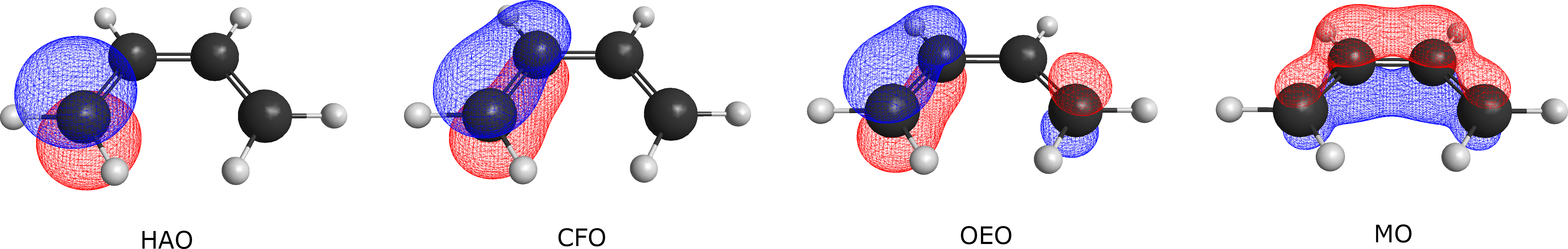
Fig. 3.2.1 Comparison of different orbital types in C4 H6
In this section, we will introduce the types of orbitals that are commonly encountered in VB calculations and discuss their characteristics.
3.2.1. Hybrid Atomic Orbital (HAO)
HAO is a type of strictly localized valence bond orbital. Such orbitals are strictly localized on a certain atom or group, and do not have any distribution on other atoms or groups, even if they are adjacent. A typical example of HAO is the hydrogen atomic orbital or the orbital localized on the CH3 group in C2 H6. HAO is the orbital type that best reflects the classical valence bond theory. Valence bond structures constructed with HAO exhibit well-defined covalent/ionic character, which is most helpful for analyzing chemical bonds.
3.2.2. Coulson-Fischer Orbital (CFO)
HAO has the advantage of a clear chemical interpretation, but the drawback is that it usually leads to a large computational cost. For systems that are even moderately larger, HAO often involves a larger number of valence bond structures and orbitals, which significantly increases the computational workload. To obtain a more compact valence bond wave function and thereby reduce the computational effort, Coulson and Fischer proposed a more delocalized orbital, the CFO. Compared with HAO, a CFO also has distribution on neighboring atoms/groups. For example, in H2, if \(\varphi_{\textrm{H}_1}\) and \(\varphi_{\textrm{H}_2}\)are the atomic orbitals of the two hydrogen atoms (i.e., HAOs), then CFO can be expressed as:
As can be seen, a CFO is essentially an HAO that delocalizes toward neighboring atoms/groups, and thus belongs to the category of semi-localized orbitals. In the case of H2, if valence bond structures are constructed with HAOs, there are three VB structures: one covalent and two ionic. However, if CFOs are used, we end up with only one covalent-type VB structure, which encompasses all three VB structures under the HAO scheme.
CFOs can reduce computational cost while maintaining accuracy of the final result. However, they sacrifice the clarity of the chemical picture inherent in valence bond structures, since covalent and ionic characters are now merged and cannot be distinguished.
3.2.3. Overlap Enhanced Orbital (OEO)
If CFOs are further delocalized, such that orbitals are delocalized over all atoms/groups in the entire system, then we obtain OEOs. OEOs are fully delocalized orbitals. At this point, VB structures no longer retain a clear chemical picture, so it is not possible to analyze chemical bonds directly based on OEO-constructed structures. However, due to orbital delocalization, the energy obtained from OEO calculations is usually the lowest. It can be mathematically proven that, within the same active space, VB calculations employing all structures with OEOs yield the same energy as CASSCF in molecular orbital theory.
It should be emphasized that although OEOs and molecular orbitals are both delocalized over the entire system, OEOs are not molecular orbitals. The delocalization of molecular orbitals is determined by symmetry, and their shapes usually reflect the intrinsic symmetry of the system. By contrast, an OEO originates from a particular atom or group and then delocalizes to other atoms or groups, and is essentially still an atomic orbital.
3.3. Methods for Constructing Valence Bond Orbitals in XMVB
3.3.1. The Simplest: Directly Specifying Basis Functions
The simplest construction method is to directly specify the basis functions included in each valence bond orbital. For instance, for the H2 molecule in the 6-31G basis set, the molecular orbital information is:
1                  1          2          3          4
2               -0.5958     0.2385     0.7747     1.4044
3                  A          A          A          A
4 1  H  1  S    0.326935   0.122649   0.766315   1.122635
5 2  H  1  S    0.271806   1.714895  -0.686252  -1.349432
6 3  H  2  S    0.326935  -0.122649   0.766315  -1.122635
7 4  H  2  S    0.271806  -1.714895  -0.686252   1.349432
We can see that under the 6-31G basis set, each hydrogen atom has two \(s\) -type basis functions. Thus, if we want to construct HAO-type VB orbitals, we can write the orbital specification part as:
1$ORB
22 2
31 2
43 4
5$END
In $ORB, the first line 2 2 means each valence bond orbital consists of two basis functions, and the next two lines 1 2 and 3 4 specify that the two VB orbitals are composed of basis functions 1 2 and 3 4, respectively. Combining with the basis set information, we know these two VB orbitals are HAOs, strictly localized on individual hydrogen atoms. If we switch the basis set to cc-pVDZ, the $ORB section must be modified accordingly. Since under cc-pVDZ, each H atom has five basis functions (S, S, PX, PY, PZ), the $ORB section would become:
1$ORB
25 5
31 2 3 4 5
46 7 8 9 10
5$END
Going a step further, if we assume the H–H bond lies along the z-axis, then PX and PY basis functions contribute nothing to H–H bonding. We can exclude them when constructing VB orbitals, and then $ORB can be modified as:
1$ORB
23 3
31 2 5
46 7 10
5$END
As can be seen, directly specifying basis functions is a simple and intuitive way to construct VB orbitals. However, for larger systems this method leads to overly lengthy and complex orbital specifications. Moreover, for the same system, whenever the basis set changes, the orbitals need to be redefined. In practice, calculations often involve multiple basis sets, which makes this method inconvenient. In early versions of XMVB, direct basis specification was the only construction method. Even today, it remains the default method in XMVB. Later, we introduced other methods to simplify the construction of VB orbitals.
3.3.2. Constructing Valence Bond Orbitals by Specifying Atoms
Since valence bond theory emphasizes chemical bonding between atoms and groups, and since VB orbitals are localized on atoms or groups (which are themselves composed of atoms), it is natural to consider whether VB orbitals can be described by directly specifying the atoms on which they are localized. In XMVB, this can be achieved by using keywords to construct VB orbitals through atom specification. Once the atoms involved in the localized orbitals are specified, XMVB automatically includes all basis functions on those atoms as components of the orbital. For example, for the H2 molecule, we can use the following form to define orbitals based on the atoms involved (here we only keep the keywords related to orbital definition):
1$CTRL
2ORBTYP=HAO FRGTYP=ATOM
3$END
4$ORB
51 1
61
72
8$END
In this example, the keywords ORBTYP=HAO FRGTYP=ATOM instruct XMVB to construct VB orbitals by specifying the atoms on which the orbitals are localized. In the $ORB section, the first line 1 1 indicates that each of the two orbitals is localized on one atom. The following two lines specify that the two orbitals are localized on atom 1 and atom 2, respectively. Similarly, for the ethane molecule C2 H6, if we want to localize the orbitals on the two CH3 groups, we can define them as:
 1$CTRL
 2ORBTYP=HAO FRGTYP=ATOM
 3$END
 4$ORB
 54 4 4 4 4 4 4 4 4 4
 61 2 3 4
 75 6 7 8
 81 2 3 4
 95 6 7 8
101 2 3 4
115 6 7 8
121 2 3 4
135 6 7 8
141 2 3 4
155 6 7 8
16$END
In this definition, each VB orbital is localized on one CH3 group, so the orbitals localized on the same group are described identically. Compared to the direct basis-function specification method, this approach is more concise and is adaptable to any basis set. Regardless of which basis set is used in the calculation, the orbital specification remains unchanged. However, this method cannot accurately describe the symmetry of the orbitals—or more informally, the “shape” of the orbitals. In practice, it is often necessary to provide a reasonably good initial guess to ensure smooth convergence of the calculation.
3.3.3. Constructing Valence Bond Orbitals Using the Symmetry of Basis Functions
If the system under study possesses well-defined symmetry, we can also use that symmetry to group the basis functions, and then construct VB orbitals from these groups. This method is referred to as the Symmetrized Atomic Orbital (SAO) method. A typical example is the HF molecule, which is a heteronuclear diatomic molecule. If we place the bond axis along the z-axis, we can, based on the molecular symmetry, classify the basis functions into three groups:
Basis functions with the same symmetry as a σ bonding orbital, such as \(s\) ,\(p_z\) , \(d_{xx}\) , \(d_{yy}\) , \(d_{zz}\)etc.;
Basis functions similar to \(p_x\) , such as \(p_x\) , \(d_{xz}\);
Basis functions similar to \(p_y\) , such as \(p_y\) , \(d_{yz}\)
In this way, the basis functions on the atoms can be grouped according to their symmetry, and these groups are then used to construct VB orbitals. The orbital input for HF molecule is:
 1$CTRL
 2ORBTYP=HAO FRGTYP=SAO
 3$END
 4$FRAG
 51 1 1 1
 6spzdxxdyydzz 2
 7pxdxz 2
 8pydyz 2
 9s 1
10$END
11$ORB
121 1 1 1 1 1
131
141
152
163
171
184
19$END
20$GEO
21H 0.0 0.0 0.0
22F 0.0 0.0 1.0
23$END
我们看到,此时关键词变成了 FRGTYP=SAO ,表明我们需要利用 SAO 方法来构建价键轨道。同时,输入文件中出现了一个新的模块 $FRAG 。这个模块用于描述基函数的分组情况。在 HF 分子的例子中,我们将基函数分为了 4 组,每组包含 1 个原子上的基函数,这就是第一行 1 1 1 1 的含义。接下来 4 行分别定义了每个组内的基函数。每一行有两部分内容,内容间用空格隔开。第一部分内容描述了组内的基函数(这部分内容内没有空格),第二部分描述了这些基函数在哪些原子上,可以用空格隔开多个原子。比如,第一行 spzdxxdyydzz 2 ,我们可以将它分解为 spzdxxdyydzz 和 2 两部分内容。第一部分内容表示这组基函数包括了 \(s\) , \(p_z\) , \(d_{xx}\) , \(d_{yy}\) 和 \(d_{zz}\) 基函数,第二部分表示这些基函数在第二个原子(根据 $GEO 中的内容,可以知道这个原子是 F 原子)上。综合来看, spzdxxdyydzz 2 表示这组基函数包含了第二个原子( F 原子)上的 \(s\) , \(p_z\) , \(d_{xx}\) , \(d_{yy}\) 和 \(d_{zz}\) 基函数。同样,第二行表示这一组包含了 F 原子上的 \(p_x\) 和 \(d_{xz}\) 基函数;第三行表示这组包含了 F 原子上的 \(p_y\) 和 \(d_{yz}\) 基函数;最后一组表示 H 原子上的 \(s\) 基函数。
With the basis function groups defined, we can then construct VB orbitals in $ORB using these groups. In $ORB, the first line 1 1 1 1 1 1 specifies that there are six orbitals, each built from one group of basis functions. Each subsequent line specifies which group forms each orbital. From the $FRAG definition, it is clear that orbital 3 corresponds to F’s \(p_x\)orbital, orbital 4 corresponds to F’s \(p_y\)orbital, the last orbital corresponds to H’s \(s\)orbital, orbitals 1, 2, and 5 are the \(\sigma\)-space orbitals on the F atom, which can be readily identified as \(1s\), \(2s\), and the \(\sigma\)bonding orbital primarily composed of \(p_z\).
Another example is ethylene ( C2 H4 ). This is a typical planar molecule. Suppose the molecule lies in the XY plane, with the \(\pi\)orbitals oriented along the \(p_z\)direction. If we are only interested in the active space of the \(\pi\)orbitals, then the \(\sigma\)bonds within the XY plane are irrelevant to our problem. We can thus delocalize the \(\sigma\)space completely (keeping the MO character), and only construct localized orbitals for the \(\pi\)space. Therefore, we can divide the basis functions into two groups:
In-plane (XY) basis functions belonging to the \(\sigma\)space, such as \(s\) , \(p_x\) , \(p_y\) , \(d_{xx}\) , \(d_{yy}\) , \(d_{zz}\), \(d_{xy}\), etc;
Out-of-plane basis functions belonging to the \(\pi\)space, such as \(p_z\) , \(d_{xz}\) , \(d_{yz}\), etc.
Since we only construct localized orbitals for the second group, the input for VB orbitals is:
 1$CTRL
 2ORBTYP=HAO FRGTYP=SAO
 3$END
 4$FRAG
 56 1 1
 6spxpydxxdyydzzdxy 1 2 3 4 5 6
 7pzdxzdyz 1
 8pzdxzdyz 4
 9$END
10$ORB
111 1 1 1 1 1 1 1 1
121
131
141
151
161
171
181
192
203
21$END
Here, the $FRAG block divides the basis functions into three groups: the first group consists of \(\sigma\)-space basis functions from all atoms, used to construct delocalized orbitals; the second and third groups correspond to the \(\pi\)-space basis functions of the two carbon atoms, used to construct localized active orbitals. In $ORB, the first seven orbitals are built from the first group, representing non-active \(\sigma\)-space orbitals, while the last two orbitals correspond to localized \(\pi\)-space active orbitals.
The SAO method thus provides a degree of flexibility and adapts well to different basis sets. Compared with directly specifying basis functions, the input file is simpler; compared with the atom-specification method, SAO reduces the demand for good initial guesses by incorporating symmetry, making it more robust. However, SAO is advantageous only when the system has reasonably high symmetry and the basis functions can be grouped accordingly. For systems with low symmetry, or when the relevant basis functions cannot be grouped by symmetry, SAO is not a particularly efficient method.