6. Excited States

Up to this point, our focus has been on ground-state calculations. In real research tasks, however, molecules cannot always remain in the ground state, and researchers’ interests are not confined to ground-state properties alone. Therefore, in this section we will briefly discuss how to carry out calculations of excited states.

6.1. Different Pictures of Excited States in MO and VB Theories

In MO theory, atomic orbitals are linearly combined to form molecular orbitals. Each molecular orbital has its own energy, and electrons occupy orbitals according to the aufbau principle, i.e., filling them from lowest to highest energy. In the case of orbital degeneracy, Hund’s rule applies: electrons are first distributed with parallel spins among the degenerate orbitals before pairing up. The electronic state obtained in this manner is typically the ground state, since all unoccupied orbitals are of higher energy than the occupied ones. If, however, electron occupation does not follow these rules—for example, if in degenerate orbitals one orbital is filled completely before occupying the others, or if a higher-energy orbital is filled while a lower-energy orbital remains empty or only partially filled—the total energy of the molecule increases. The resulting higher-energy state is what we call an excited state. Such states are unstable and are usually formed when electrons in a ground-state molecule absorb some form of energy (e.g., photons), which promotes them into higher-energy orbitals or configurations. In MO theory, the excitation energy of a molecule can be roughly estimated by Koopmans’ theorem, namely

\[E_i^a = \varepsilon_a - \varepsilon_i\]

In actual calculations, however, because orbital occupation changes after excitation, the orbitals themselves undergo relaxation. Therefore, the true excitation energy must take orbital relaxation into account, and a self-consistent field iteration is required.

In VB theory, the molecular wavefunction is determined by two aspects: the choice of orbitals that define the resonance structures, and the linear combination of these structures. Different orbital choices correspond to different physical meanings and chemical pictures of the resonance structures, while different combination coefficients yield different properties and states of the molecule. The combination coefficients are obtained by solving the secular equation. For a molecule with n structures, the secular equation corresponds to an n-dimensional generalized eigenvalue problem, which yields n solutions in total. The first solution corresponds to the lowest-energy combination. When orbital occupations follow the aufbau principle, this first root corresponds to the ground state of the molecule. If we do not take the first root, or if the electron occupations do not follow the lowest-energy filling, the resulting combination of structures changes, and we obtain an excited state. We can see here that excited-state calculations in VB theory involve two dimensions: the choice of orbitals and the variation in combination coefficients. Since orbital choices determine the specific physical meaning and chemical picture of the resonance structures, please refer back to Section 2 and Section 3. In this lecture, our focus will be on how changes in combination coefficients affect excited states.

6.2. How to Calculate Excited States in XMVB

6.2.1. Obtaining Specific Excited States

XMVB provides the keyword NSTATE=IROOT to select different roots of the secular equation, where IROOT is a non-negative integer indicating which excited state to compute. NSTATE=1 means the program will select the second root to obtain the first excited state, NSTATE=2 corresponds to the second excited state, and so forth. NSTATE=0 specifies the ground-state (zeroth excited state) calculation, which is also the default.

Let us first look at the H₂ molecule to see the effect of NSTATE=IROOT. By default, XMVB performs a ground-state calculation. For an H–H bond length of 0.7 Å with the cc-pVDZ basis set in an HAO calculation, the energy obtained is –1.14386 a.u., and the coefficients and weights of the three valence-bond structures are as follows:

           ******  COEFFICIENTS OF STRUCTURES ******

    1      -0.84426638  ******    1-2
    2      -0.09228443  ******    1 1
    3      -0.09228443  ******    2 2


          ******  WEIGHTS OF STRUCTURES ******

    1       0.84327776  ******    1-2
    2       0.07836112  ******    1 1
    3       0.07836112  ******    2 2

Here, the covalent structure clearly dominates. If we add NSTATE=1, the final energy becomes –0.38420 a.u., and the corresponding structure coefficients and weights are:

           ******  COEFFICIENTS OF STRUCTURES ******

    1      -0.00000000  ******    1-2
    2       1.51521437  ******    1 1
    3      -1.51521436  ******    2 2


          ******  WEIGHTS OF STRUCTURES ******

    1       0.00000000  ******    1-2
    2       0.50000000  ******    1 1
    3       0.50000000  ******    2 2

We can see that the covalent structure has vanished, and the coefficients of the ionic structures have changed from equal to opposite. This corresponds to the coefficients of the first excited state.

Next, let us consider a more complex example: ₂O₂. The triplet state of O₂ requires 12 resonance structures, while the singlet state requires 10. The 12 structures of the triplet state are shown in Fig. 6.2.1, with T1 and T2 being the most important.

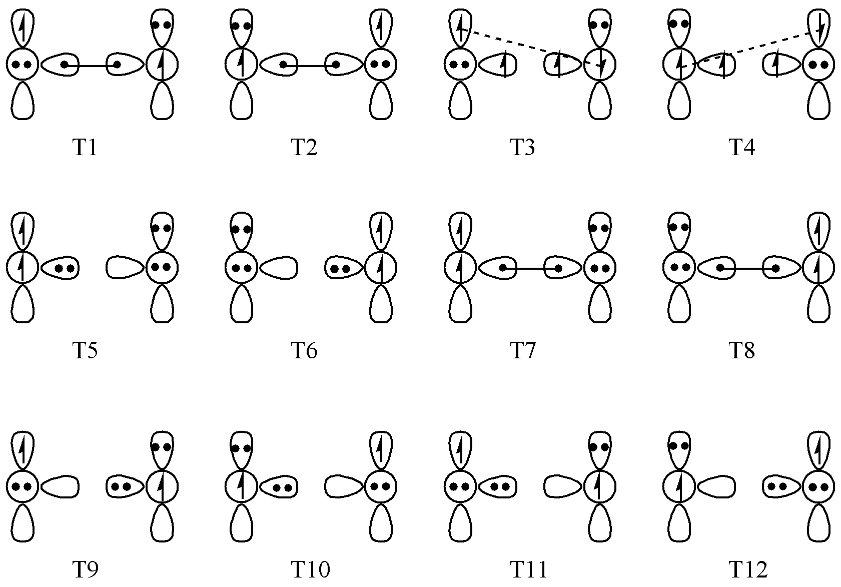
Fig. 6.2.1 The 12 valence-bond structures of triplet O₂

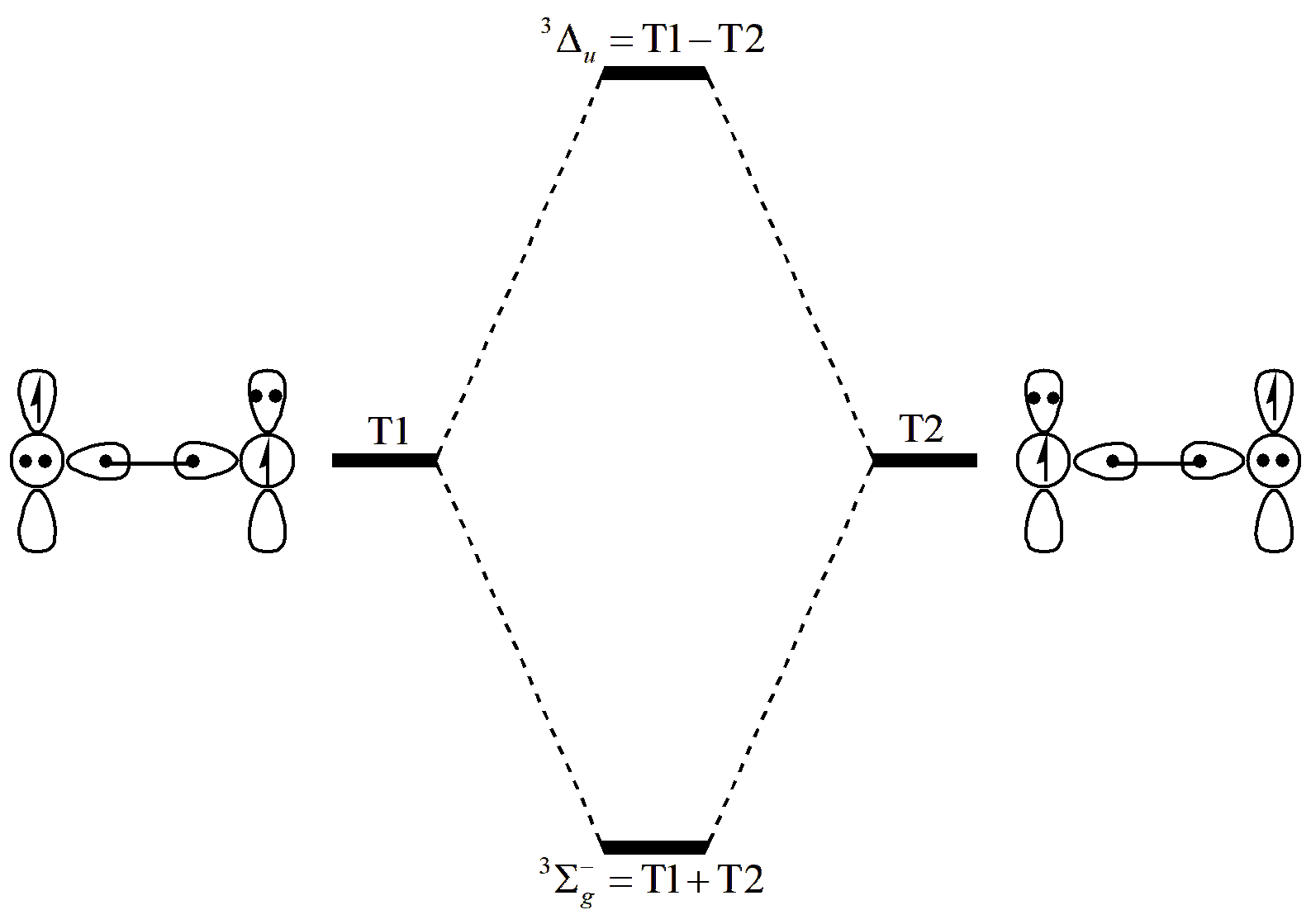
Fig. 6.2.2 The ground and excited states of triplet O₂

As shown in Fig. 6.2.2, different combinations of T1 and T2 correspond to different electronic states. In the ground state, the coefficients of these two structures are the same; in the excited state, the coefficients are opposite.

To obtain the excited state of the triplet, we can compute the first excited state by setting NSTATE=1, as shown below:

O2 L-VBSCF
$ctrl
vbscf nstr=12 nao=6 nae=8 iscf=5 iprint=3
orbtyp=hao frgtyp=sao nmul=3 itmax=200 nstate=1
int=libcint basis=cc-pvdz
guess=read
$end
$str
1:4 7 7 10 10 5 6 8 9
1:4 8 8 9 9 5 6 7 10
1:4 7 7 10 10 8 9 5 6
1:4 8 8 9 9 7 10 5 6
1:4 7 7 9 9 5 6 8 10
1:4 8 8 10 10 5 6 7 9
1:4 8 8 10 10 5 5 7 9
1:4 7 7 9 9 6 6 8 10
1:4 8 8 9 9 5 5 7 10
1:4 7 7 10 10 6 6 8 9
1:4 7 7 10 10 5 5 8 9
1:4 8 8 9 9 6 6 7 10
$end
$frag
1*6
spzdxxdyydzzfzzzfxxzfyyz 1
spzdxxdyydzzfzzzfxxzfyyz 2
pxdxzfxxxfxyyfxzz 1
pxdxzfxxxfxyyfxzz 2
pydyzfyyyfxxyfyzz 1
pydyzfyyyfxxyfyzz 2
$end
$orb
1*10
1
2
1
2
1
2
3
4
5
6
$end
$geo
O 0.0 0.0 0.0
O 0.0 0.0 1.2
$end
$gus
    8    8    8    8    8    8    3    3    3    3
 1.0019774038    1   0.0065168066    2   0.0001788772    3   0.0010309980    6
-0.0003633198    9  -0.0027414664   10  -0.0030686413   13  -0.0030026561   15
 1.0021643892   16   0.0072505362   17   0.0002382456   18  -0.0011188449   21
 0.0003834680   24  -0.0030102480   25  -0.0031503232   28  -0.0032525782   30
 0.0982223750    1  -0.2504910231    2  -0.8206750714    3  -0.0401288970    6
-0.3250457745    9   0.0663093980   10   0.0645475585   13  -0.0255293114   15
 0.1023941578   16  -0.2356452123   17  -0.8258612653   18   0.0419646005   21
 0.3491578062   24   0.0683659578   25   0.0684486346   28  -0.0278018600   30
-0.0534466425    1  -0.2957625003    2  -0.0041914149    3   0.2677956458    6
 0.7578794938    9  -0.0782023209   10  -0.0786400588   13   0.0255903120   15
-0.0521455763   16  -0.3057336084   17  -0.0199773005   18  -0.2554552086   21
-0.7557006120   24  -0.0788914259   25  -0.0791889215   28   0.0231651215   30
 0.5315910156    4   0.6213802169    7   0.0117253831   12
 0.5179245322   19   0.6342323659   22  -0.0135520711   27
 0.5280659286    5   0.6247144659    8   0.0122018946   14
 0.5244186959   20   0.6281355341   23  -0.0136783062   29
$end

Compared with the ground-state calculation, the only change in the input file is the inclusion of the NSTATE keyword. Removing NSTATE=1 reverts the calculation to the ground state. The final results are given in Table 6.2.1:

Table 6.2.1 Valence-bond wavefunctions of triplet O₂ in the ground and excited states

Structure	Ground State		Excited State
	Coefficient	Weight	Coefficient	Weight
T1	-0.343	0.220	-0.492	0.327
T2	-0.343	0.220	0.492	0.327
T3	-0.018	0.000	-0.036	0.001
T4	0.018	0.000	-0.036	0.001
T5	0.166	0.073	0.000	0.000
T6	0.166	0.073	0.000	0.000
T7	0.178	0.091	0.000	0.000
T8	0.178	0.091	0.000	0.000
T9	-0.125	0.058	-0.180	0.086
T10	-0.125	0.058	0.180	0.086
T11	-0.125	0.058	-0.180	0.086
T12	-0.125	0.058	0.180	0.086

From these results, we can see that the combination of coefficients of T1 and T2 indeed changes between the ground and excited states. We also see that, both in terms of coefficients and weights, the excited state is dominated by T1 and T2, with diminished contributions from the other structures. The first excited state of triplet O₂ is thus primarily composed of the two structures T1 and T2.

6.2.2. State-Averaged Calculations

When performing excited-state calculations, it is often useful to employ state averaging. In a state-averaged calculation, we do not optimize a single electronic state. Instead, we combine the energies of several states of interest according to predefined weights, and then use self-consistent field iterations to optimize the orbitals such that the weighted total energy is minimized:

\[E = \sum_i{w_iE_i}\]

where \(E\) is the total energy, \(E_i\) is the energy of a particular state included in the state averaging, and \(w_i\) is the corresponding weight, which remains fixed during the optimization.

In XMVB, the keyword WSTATE is used to perform state-averaged calculations. Its syntax is:

WSTAE( start )= \(w_{\textrm{start}}\), \(w_\textrm{start+1}\), …

Here, start in parentheses denotes the index of the first state included. The ground state is indexed as 1, the first excited state as 2, and so forth. The numbers after the equals sign, separated by commas, specify the weights of consecutive states. For example:

WSTATE(1)=0.4,0.6

performs a two-state average, where the ground state has weight 0.4 and the first excited state has weight 0.6. Multiple WSTATE keywords can also be combined, for example:

WSTATE(1)=0.5,0.5 WSTATE(5)=0.4,0.6

Here, the state averaging involves four states: the ground state (weight 0.5), the first excited state (weight 0.5), the fourth excited state (weight 0.4), and the fifth excited state (weight 0.6). Note that the sum of weights here is greater than 1. XMVB automatically normalizes the weights to unity, so the above input is equivalent to:

WSTATE(1)=0.25,0.25 WSTATE(5)=0.2,0.3

Users only need to focus on the ratios between the weights of different states. The default value of WSTATE is

WSTATE(1)=1.0,0.0,0.0, ...

Which means only the ground state is optimized. State-averaged calculations can be applied in both VBSCF and BOVB computations. As an example, consider H₂. We perform a state-averaged calculation involving the ground state and the first excited state, with weights of 0.7 and 0.3, respectively. The input file is:

H2 State average
$ctrl
vbscf
str=full nao=2 nae=2 iscf=5
orbtyp=hao frgtyp=atom
int=libcint basis=cc-pvdz
wstate(1)=0.7,0.3
$end
$orb
1*2
1
2
$end
$geo
H 0.0 0.0 0.0
H 0.0 0.0 0.74
$end

In the output file, we see a message confirming that this is a state-averaged calculation:

  Stat average computation with folllowing states and weights:

   STATE     WEIGHT
     1       0.700
     2       0.300

Finally, in addition to the total energy, XMVB also outputs the energy, structure coefficients, and weights for each individual state included in the averaging. For example, the ground-state information is:

         STATE:     1
         ENERGY:      -1.13344128
         WEIGHT:       0.70000000

         ******  COEFFICIENTS OF STRUCTURES ******

  1      -0.90250405  ******    1-2
  2       0.05647560  ******    1 1
  3       0.05647560  ******    2 2


        ******  WEIGHTS OF STRUCTURES ******

  1       0.90219477  ******    1-2
  2       0.04890261  ******    1 1
  3       0.04890261  ******    2 2